Google Apps: Applying Conditional Formatting Across Sheets
Common wisdom says you just can't apply conditional formatting in a Google Apps spreadsheet using data from a different sheet. But here at Campus Technology, we laugh in the face of wisdom, common or otherwise. But is such jocularity justified? Read on.
|
Long Story Short
For you advanced users who want to skip ahead: You apply the conditional formatting using a custom formula and some variation on the INDIRECT function. In addition to specifying the column and row, you also specify the name of the sheet to pull the data from ("Sheet2," for example).
Here's a sample formula you can try on your own:
=if((INDIRECT("Sheet2!A"&ROW()))>1,1,0)=1
That says if a number in Sheet2, column A, corresponding row (dynamically called in this case) is greater than 1, the apply the format specified (text and background color).
|
The problem: Using conventional techniques, conditional formatting allows you to specify a range of cells that will determine the formatting within the same spreadsheet; the data usually cannot be taken from multiple sheets within the spreadsheet. So, for example, if you're working in Sheet1, then all of your formatting is applied to Sheet1 only.
But what if you want to format cells in Sheet1 based on values that appear in Sheet2?
There is a workaround. It involves something we've covered in the past — custom formulas — coupled with data calls that cut across sheets.
Cross-Sheet Data Calls
Google Sheets fully supports calling data from one sheet and using it in another. It's very simple using the INDIRECT function (and other means) and dynamic cell calls (which we covered extensively in our previous tutorial). Try it out.
1. Make sure you have at least two sheets in your spreadsheet. You can create sheets by clicking the "+" button at the bottom of your browser window.

2. In Sheet1, type this formula into any cell in column A:
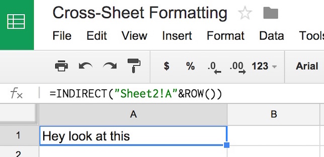
=INDIRECT("Sheet2!A"&ROW())
Using the exclamation point between the name of the sheet and the column and row reference, this formula displays in a cell in Sheet1 whatever is in Sheet2 in column A in the corresponding row. ("&ROW()" inserts the number of the current row into the formula dynamically, so you could apply this formula to every cell in column A without modification. Data from the corresponding row in Sheet2 will be displayed in each cell in Sheet1 to which you've applied this formula. In our next tutorial, I'll show you how to work dynamic column calls into an INDIRECT expression as well. It's a little more involved.)
3. Now in Sheet2, type a number or some text in the corresponding cell. I'll type "Hey look at this" into cell A1 in Sheet2. The same text will now show up in cell A1 in Sheet1. And it will be automatically updated in Sheet1 whenever I change the text in Sheet2.
Adapting This Trick for Conditional Formatting
Now, just as we learned last time around, we can use "if" statements in concert with the INDIRECT function to apply conditional formatting by using the "Custom formula" option in the Conditional Formatting dialog.
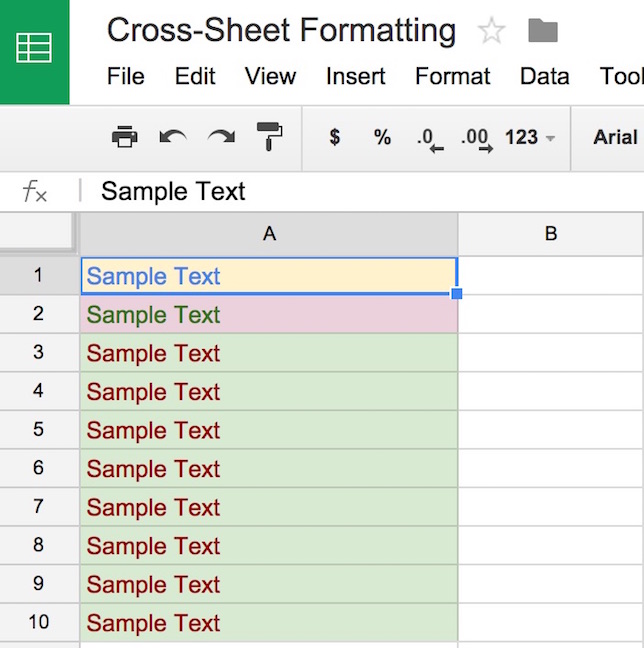
For my example, I'm going to have the first 10 cells in Sheet1, column A use conditional formatting based on numeric values in the corresponding cells in Sheet2.
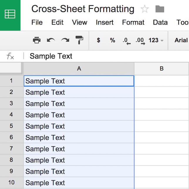
Here are my unformatted cells in Sheet1.
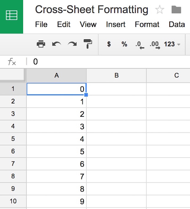
Now, in Sheet2, I'm going to put in some arbitrary numeric values, from 0 to 9.
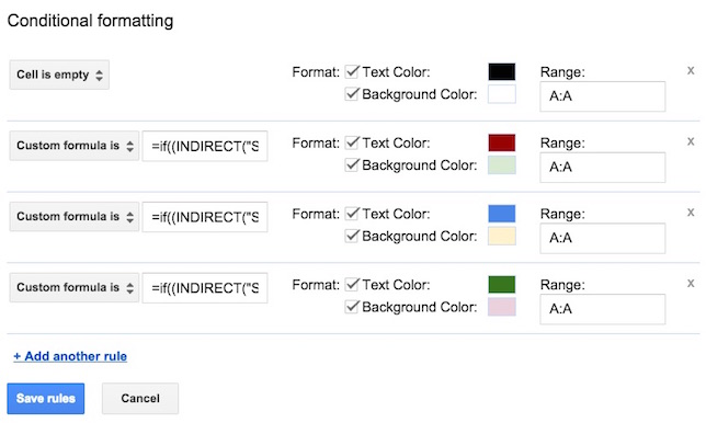
Now I'm ready to apply my conditional formatting. I'm going to create four rules — three of them using the "Custom formula is" option. I will apply these to the entire column A by clicking the letter A at the top of the column and selecting Format > Conditional formatting.
1. For empty cells, I'm going to specify that their backgrounds will remain white. (This must be the first rule in the list. Create it first; as of this writing, you can't reorder your rules once they're created.)
2. My second rule will be a custom formula that looks for any number larger than 1 in the corresponding cell in Sheet2. That's this formula:
=if((INDIRECT("Sheet2!A"&ROW()))>1,1,0)=1
3. My third rule will be based on any number smaller than 1. That's this formula:
=if((INDIRECT("Sheet2!A"&ROW()))<1,1,0)=1
4. And my fourth will look for any number equal to 1. That's this formula:
=if((INDIRECT("Sheet2!A"&ROW()))=1,1,0)=1
Here's how that looks in the Custom Formatting dialog.
Click the "Save rules" button, and voila! The formatting in Sheet1 is set based on conditions in Sheet2. And that formatting will update itself automatically whenever the data in Sheet2 changes.
That's all there is to it. There are limitless variations you can apply using this basic technique. However, it's worth noting that this technique is not foolproof. If there are too many of these custom formulas on a single sheet, Google Sheets may being to throw errors. (It's not clear how many are "too many." I began to see some errors when I had five different sets of conditional formats with three to four custom formulas each.) So use this technique with discretion.
Feel free to drop me a note if you need additional help.
Looking for more tutorials? Check out our Tutorial archive!