Extending Conditional Formatting in Google Sheets Using Dynamic Date Calls
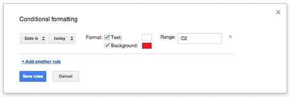
Google Sheets, the spreadsheet tool that's part of the Google Apps productivity suite, lets users format cells based on certain conditions, including the date contained in a cell and how far away that date is from the present. For example, if the date is today, the cell background can be shaded red and the text colored white, giving an immediate cue that the task due date is at hand. Tomorrow, that could change automatically to a black background, indicating the task is past due.
Yesterday and today: Conditional formatting lets users assign text and background colors based on relative dates. |
But the options available through the Conditional Formatting dialog are limited. The default options include today, tomorrow, yesterday and "exact date," along with the less useful options of "in the past week," "in the past month" and "in the past year."
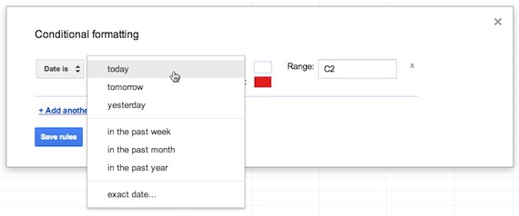
Default conditional formatting options in Google Sheets |
That doesn't give a lot of options for providing visual cues about date-based information, such as how far in the future a particular assignment might be due.
But there is, in fact, a workaround for this that will allow you to assign text and background colors based on any date in the future that you choose to assign — eight days from now, 21 days from now, whatever. You just have to borrow a simple formula commonly used in other spreadsheets.
It works like this:
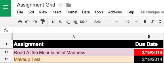
1. Select your entire column or the range of cells to which you want to apply the formatting, then choose Format > Conditional Formatting. In my case, I will choose the "Due Date" column in my assignment spreadsheet for a hypothetical H.P. Lovecraft seminar (since I happen to be wearing my Miskatonic U sweatshirt as I write this).
2. Click the "+Add Another Rule" button.
3. In the pull-down menu, instead of choosing "Date Is," choose "Is Equal to."
4. Then enter the following formula:
=TODAY() +3
That indicates a date that is three days in the future from the present (whatever the present date happens to be when the user is viewing the spreadsheet).
Repeat that step for all of the possible dates that you want to format. For four days hence, use
=TODAY() +4
For five days hence, use
=TODAY() +5
Et cetera.
5. Apply the text and background colors of your choosing to all of the options you've created. I will set mine to become progressively cooler (greens and blues) the further the due date is in the future and warmer (yellows and reds) as the due date nears.
Click the Save button, and voila!
You wind up with a very colorful spreadsheet with immediately identifiable date cues.
Next time: conditional formatting based on ranges.