Formatting Cells Based on Date Ranges in Google Sheets
|
Conditional Formatting
In Google Sheets, as in other spreadsheet programs, you can set the formatting of a cell (text color, background color) based on the data contained within that cell. This is called "conditional formatting," and it's valuable in that it provides visual cues for your users. A red cell, for example, might indicate an impending sue date. The data can include dates, text and numbers.
|
In our first tutorial on Google Sheets, we looked at extending the software's default conditional formatting options through the use of formulas. That solution is good for a limited range of dates, but it might get cumbersome in spreadsheets that span longer periods, since each possible date requires a unique formula.
But there is a way to simplify the conditional formatting setup by using date ranges rather than individual dates.
As with last week's tutorial, begin by selecting the range of cells to which you wish to apply your conditional formatting. In my case, I want to apply my formatting to an entire column (the "Due Date" column in my example), so I'll click the top of the column to select the entire thing.
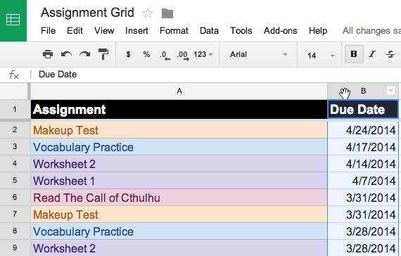
Step 1: Select the range of cells to which you wish to apply your conditional formatting. |
Then choose Format > Conditional formatting from the menu.
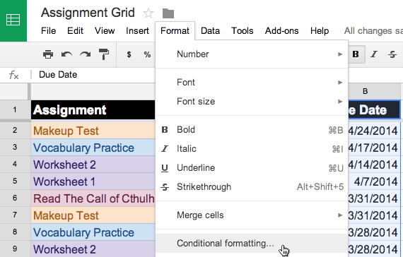
Step 2: Open the Conditional Formatting dialog. |
I'll set up four ranges of dates for my column. The ranges I'm choosing are arbitrary. You can set whatever range you want.
To begin, change the default condition ("Text contains") to "Is between." This will cause two text fields to appear. You will put your ranges inside these boxes. For my first range, I want to set anything due this week to have a red background with white text.
So in the first box, I enter the formula for today:
=TODAY() +0
And in the second box, I'll enter:
=TODAY() +7
That covers all dates from today to seven days from now.
Then change the text and background colors in the dialog.
Click "Save rules" when you're done.
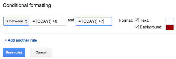
Step 3: Enter the range of dates using the same formula from last week's tutorial to define the dates. |
Now I'll repeat this for three more date ranges.
First, click "+Add another rule" for each new date range you want to create.

Step 4: Click "+Add new rule." |
Then repeat the process you used earlier, making sure that none of your dates overlap. Set colors for each range individually. In my case, I'll use cooler colors for dates that are farther away (greens and blues), hotter colors for dates that are getting closer (reds and yellows).
Click Save rules when you're done.
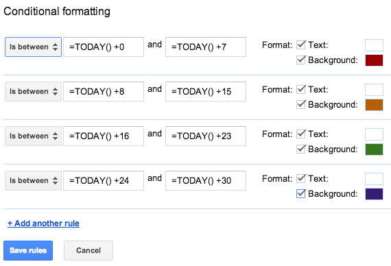
Step 5: Repeat. |
And here's the result.
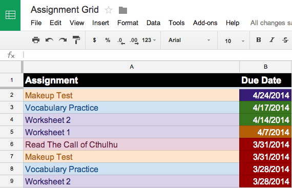
Voila! |
Next time around: extracting the date from a URL.